

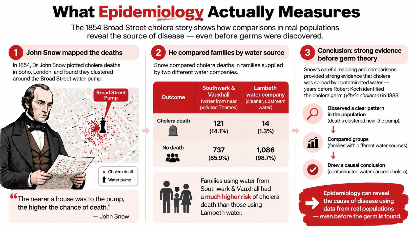
In 1854, John Snow mapped cholera deaths around London's Broad Street pump and compared households using different water sources. That simple comparison captured the heart of epidemiology: identify an exposure, count an outcome, compare groups, and decide what the pattern can reasonably prove.
What Epidemiology Actually Measures
Snow's investigation is useful because it began with a population, not a single patient. The population was people living in the affected London neighborhood. The suspected exposure was drinking water from a particular source. The outcome was cholera illness or death. The comparison group consisted of people whose water came from another supplier or source.
Snow didn't need a modern molecular explanation to ask a strong epidemiologic question. He asked whether cholera occurred differently among people exposed to different water sources. Mapping deaths helped show that cases clustered around the Broad Street pump, while household water-source information supplied a comparison. The evidence supported contaminated water as a likely cause before Koch's germ theory had been accepted.
Modern epidemiology grew from this kind of systematic observation. John Graunt's 1662 analysis of London mortality records is widely regarded as one of the first quantitative studies of disease patterns, and William Farr later systematized national mortality statistics. The CDC history of epidemiology describes how these developments helped establish vital statistics and disease surveillance.
The three primitives
Every epidemiology question gives you, explicitly or indirectly:
- A defined population: Who is being studied?
- A measured exposure: What characteristic, behavior, treatment, or environmental factor differs between groups?
- A counted outcome: What disease, event, test result, or death is being measured?
Clinical medicine often asks, “What is happening to this patient?” Epidemiology asks, “How often is this outcome occurring in a population, and how does it differ between groups?” That shift creates the language of rates, risks, ratios, and causal inference.
Practical rule: Before calculating anything, name the population, exposure, outcome, and comparison group in one sentence.
Use the same five-step workflow for nearly every quantitative question:
- Identify the question task. Is the stem asking about disease frequency, association, test performance, bias, or prevention?
- Name the study design. Determine how participants entered the study and whether observations move forward through time or describe a snapshot.
- Draw the 2×2 table. Put exposure and outcome in fixed positions before inserting numbers.
- Calculate before interpreting. Write the formula, substitute values, and simplify.
- State the result in plain English. Then ask whether prevalence, bias, confounding, or design limits the conclusion.
For a concise review of the mathematical background that supports epidemiologic analysis, see this guide to statistics for medical research. The objective isn't to memorize isolated formulas. It's to recognize which formula the study design permits.
Incidence, Prevalence, and Disease Frequency
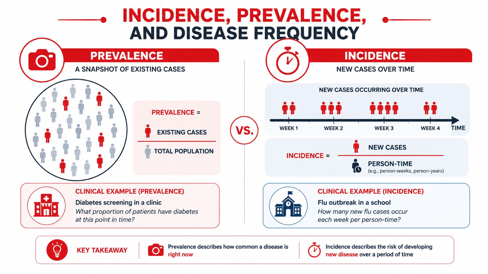
The first distinction is straightforward once you focus on time. Incidence measures new cases arising in a population during a specified period. Prevalence measures existing cases in a defined population at a particular point in time. The World Health Organization explanation of incidence and prevalence uses this distinction as a foundation for interpreting disease frequency.
Snapshot versus new occurrence
Think of prevalence as a photograph. A clinic screens a population and asks how many people currently have diabetes. The question concerns the existing burden at that moment.
Think of incidence as a video. A school follows students over a period and counts newly diagnosed influenza cases. The question concerns the emergence of new disease over time.
A bathtub analogy helps:
- Incidence is the faucet. New cases enter the pool of people with disease.
- Recovery, cure, or death is the drain. Existing cases leave that pool.
- Prevalence is the water level. It reflects both how many new cases arrive and how long people remain affected.
That's why a disease can have high incidence but modest prevalence if people recover quickly. A chronic disease can have lower incidence but substantial prevalence when affected patients remain ill for a long time.
The denominators matter
Cumulative incidence, often called risk, is the proportion of initially disease-free people who develop disease during a specified follow-up period:
Cumulative incidence = new cases during the period ÷ population at risk at the beginning
An incidence rate uses person-time:
Incidence rate = new cases ÷ total person-time at risk
Person-time is useful when participants enter at different times, leave early, or receive different durations of follow-up. Don't confuse a rate with a proportion. A proportion asks, “What fraction developed disease?” A rate asks, “How quickly did new disease arise relative to observed time?”
Two additional measures appear frequently:
- Attack rate: The proportion of an at-risk group that becomes ill during a defined outbreak or exposure event. It's a form of cumulative incidence used in outbreak settings.
- Case fatality rate: The proportion of people diagnosed with a disease who die from that disease during the specified period.
Quick classification exercise
Label each scenario as incidence or prevalence before looking at the answer:
- A survey counts the number of people currently living with asthma.
- A cohort records newly diagnosed cases of hepatitis during follow-up.
- A hospital reports the proportion of admitted patients who have pressure injuries on a particular day.
The answers are prevalence, incidence, and prevalence, respectively. Words such as “currently,” “at a given time,” and “living with” suggest a snapshot. Words such as “new,” “developed,” and “during follow-up” point toward incidence.
Study Designs and the Decision Framework
Study design determines which measure is valid. The fastest approach is to ask what investigators selected first. Did they begin with exposure, outcome, or neither? Then ask whether the study follows participants through time or captures a snapshot.
A cohort study begins with exposure status and follows participants to observe outcomes. A randomized controlled trial, or RCT, assigns an intervention or comparison condition before outcomes occur. Both can estimate risk because the denominator of people at risk is preserved.
A case-control study begins with outcome status. Investigators select people with the disease, called cases, and people without it, called controls, then look backward for exposure. Because the investigator fixes the number of cases and controls, the design generally supports an odds ratio rather than a directly calculated risk ratio.
A cross-sectional study measures exposure and outcome at one point in time. It can estimate prevalence, but timing may be unclear. If smoking and lung cancer are measured in the same survey, you may know that they coexist, but you can't confidently establish which came first.
Study design comparison
| Design | Selects On | Time Direction | Valid Measure | Strength | Weakness |
|---|---|---|---|---|---|
| Cohort | Exposure | Usually forward | Relative risk, incidence rate | Establishes temporal sequence | Can require substantial follow-up |
| Case-control | Outcome | Usually backward | Odds ratio | Efficient for uncommon outcomes | Selection and recall bias can distort findings |
| Cross-sectional | Exposure and outcome together | Snapshot | Prevalence, prevalence ratio | Describes current burden | Often cannot establish temporality |
| Randomized controlled trial | Assigned intervention | Forward | Relative risk, risk difference | Randomization balances confounders in expectation | May have ethical or practical limits |
For students who want additional statistical context beyond board-style calculations, practical regression and time series can help explain how investigators model associations and trends. That material complements, but doesn't replace, the design-first reasoning required in an exam stem.
Sketch this decision tree on scratch paper:
- Were participants selected because they had the outcome?
- Yes, case-control. Use the odds ratio.
- No, continue.
- Were participants selected by exposure or assigned an intervention?
- Yes, cohort or RCT. Risk can be calculated.
- No, continue.
- Were exposure and outcome measured at one time?
- Yes, cross-sectional. Think prevalence.
- Was an intervention assigned randomly?
- Yes, RCT.
- No, observational cohort.
The guide to critically appraising research is useful when a question asks whether the design supports the authors' conclusion. On a timed block, selection comes before arithmetic.
The 2×2 Table and Risk Measure Calculations
A 2×2 table prevents formula confusion because every cell has a fixed location. For a cohort, place exposure status in the columns and disease status in the rows.
Suppose a hypothetical cohort contains 1,000 adults, with 300 exposed to smoking and 700 unexposed, followed for five years for lung cancer. The example is deliberately constructed for practice, not presented as clinical evidence.
Labeled worksheet
| Exposed | Unexposed | Total | |
|---|---|---|---|
| Disease present | a | c | a + c |
| Disease absent | b | d | b + d |
| Total | a + b | c + d | a + b + c + d |
Here, a is disease among exposed people, b is no disease among exposed people, c is disease among unexposed people, and d is no disease among unexposed people.
| Cell | Disease Present | Disease Absent | Risk / Test Statistic |
|---|---|---|---|
| Exposed | a | b | Risk in exposed = a ÷ (a + b) |
| Unexposed | c | d | Risk in unexposed = c ÷ (c + d) |
| Exposure odds | a | b | a ÷ b |
| Unexposed odds | c | d | c ÷ d |
The first calculation is the disease frequency in each exposure group:
- Risk in exposed = a ÷ (a + b)
- Risk in unexposed = c ÷ (c + d)
Then calculate the association:
Relative risk = [a ÷ (a + b)] ÷ [c ÷ (c + d)]
A relative risk above one indicates greater observed risk in the exposed group. A value below one indicates lower observed risk. A value near one indicates little difference in risk, although confidence intervals and study validity still matter.
For an intervention that lowers risk, the absolute risk reduction is:
ARR = risk in control group − risk in treatment group
The number needed to treat is:
NNT = 1 ÷ ARR
Use the same logic when exposure increases harm:
Absolute risk increase = risk in exposed group − risk in unexposed group
NNH = 1 ÷ absolute risk increase
Keep the units consistent. If risks are written as percentages, convert the difference to a proportion before calculating NNT or NNH.
Reorienting the table for diagnostic tests
For test performance, the rows usually represent the true disease state and the columns represent the test result:
- Sensitivity = a ÷ (a + c), the proportion of people with disease who test positive.
- Specificity = d ÷ (b + d), the proportion of people without disease who test negative.
- Positive predictive value = a ÷ (a + b), the proportion of positive tests that represent true disease.
- Negative predictive value = d ÷ (c + d), the proportion of negative tests that represent true absence of disease.
Likelihood ratios combine sensitivity and specificity to update diagnostic probability. The sensitivity and specificity calculation guide offers a focused review of that test-performance framework.
Why the Odds Ratio Is Not the Relative Risk
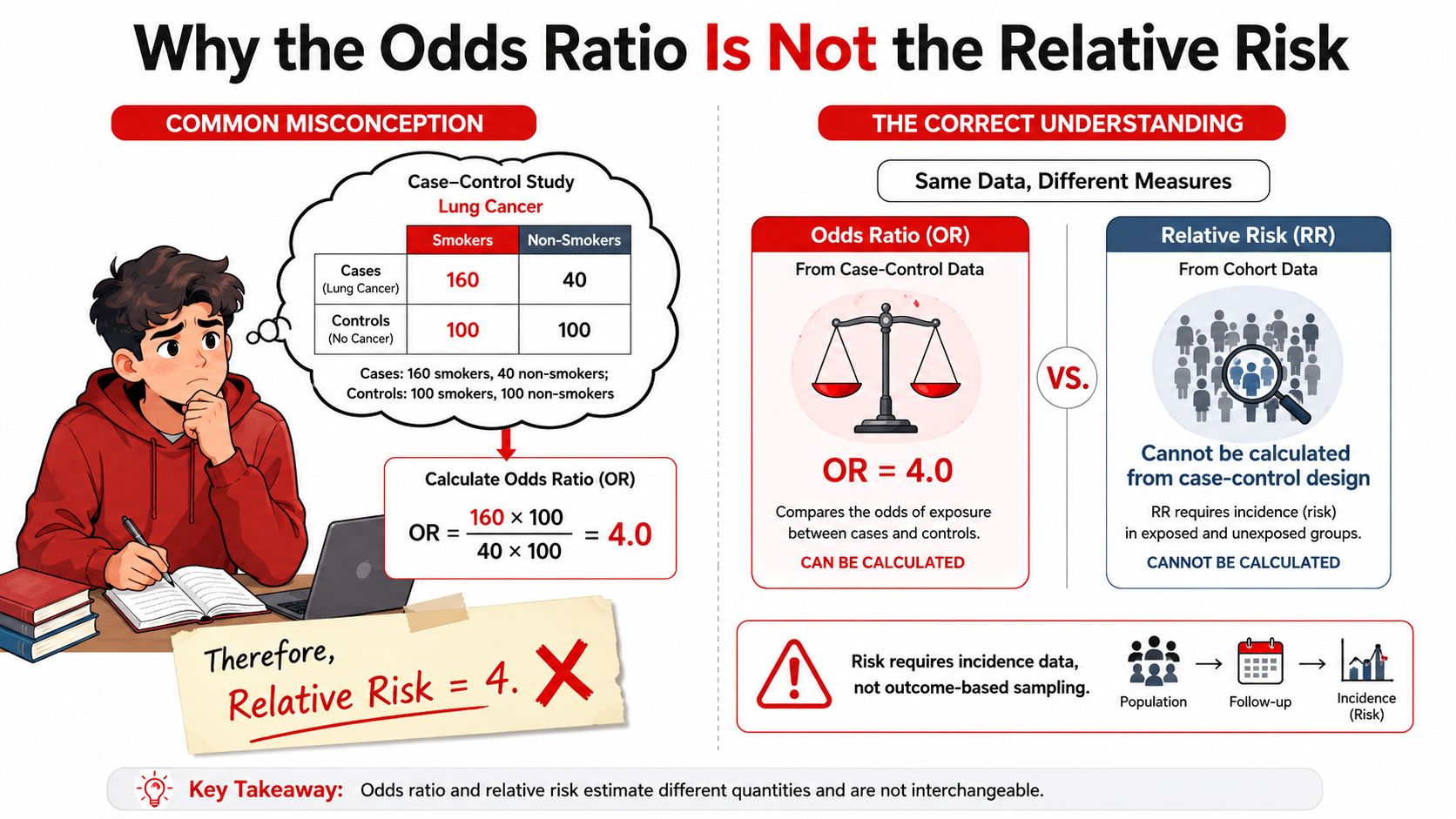
Composite learner example, clearly labeled: A learner sees a case-control vignette involving 200 lung cancer cases and 200 matched controls. Among the cases, 160 smoked and 40 did not. Among the controls, 100 smoked and 100 did not. The learner calculates an odds ratio of 4.0, then marks relative risk of 4.0.
The odds ratio calculation is valid:
OR = (a × d) ÷ (b × c)
Using the exposure counts:
OR = (160 × 100) ÷ (40 × 100) = 4.0
The error is calling that value a relative risk. The investigators selected participants according to outcome status, not exposure status. They deliberately assembled cases and controls, so the proportion of cases in the sample does not represent the proportion of disease in the exposed population.
Rebuilding the reasoning
For case-control data, compare the odds of exposure among cases with the odds of exposure among controls:
Odds of exposure among cases = a ÷ b
Odds of exposure among controls = c ÷ d
OR = (a ÷ b) ÷ (c ÷ d)
You can't directly calculate risk because the denominators needed for incidence are unavailable. The number of cases and controls was fixed by the study design, not observed naturally from exposed and unexposed populations.
Relative risk requires:
Risk in exposed = a ÷ (a + b)
Risk in unexposed = c ÷ (c + d)
In a case-control study, those denominators don't represent the original populations at risk. The odds ratio remains the appropriate association measure.
Mnemonic: OR is for outcome-first case-control studies. RR is for exposure-first cohorts and trials.
When an outcome is rare, the odds ratio can approximate the relative risk. A commonly taught board-review rule uses a prevalence below roughly 10 percent, but treat that as an approximation, not a universal law. As disease frequency rises, odds and probability separate more noticeably, so the odds ratio can increasingly exaggerate the apparent risk ratio.
Test the transfer principle mentally: the gap between OR and RR should be smaller when prevalence is 1 percent than when prevalence is 40 percent. The design still dictates the measure, and rarity determines how closely the measures may resemble each other.
Bias, Confounding, and Effect Modification
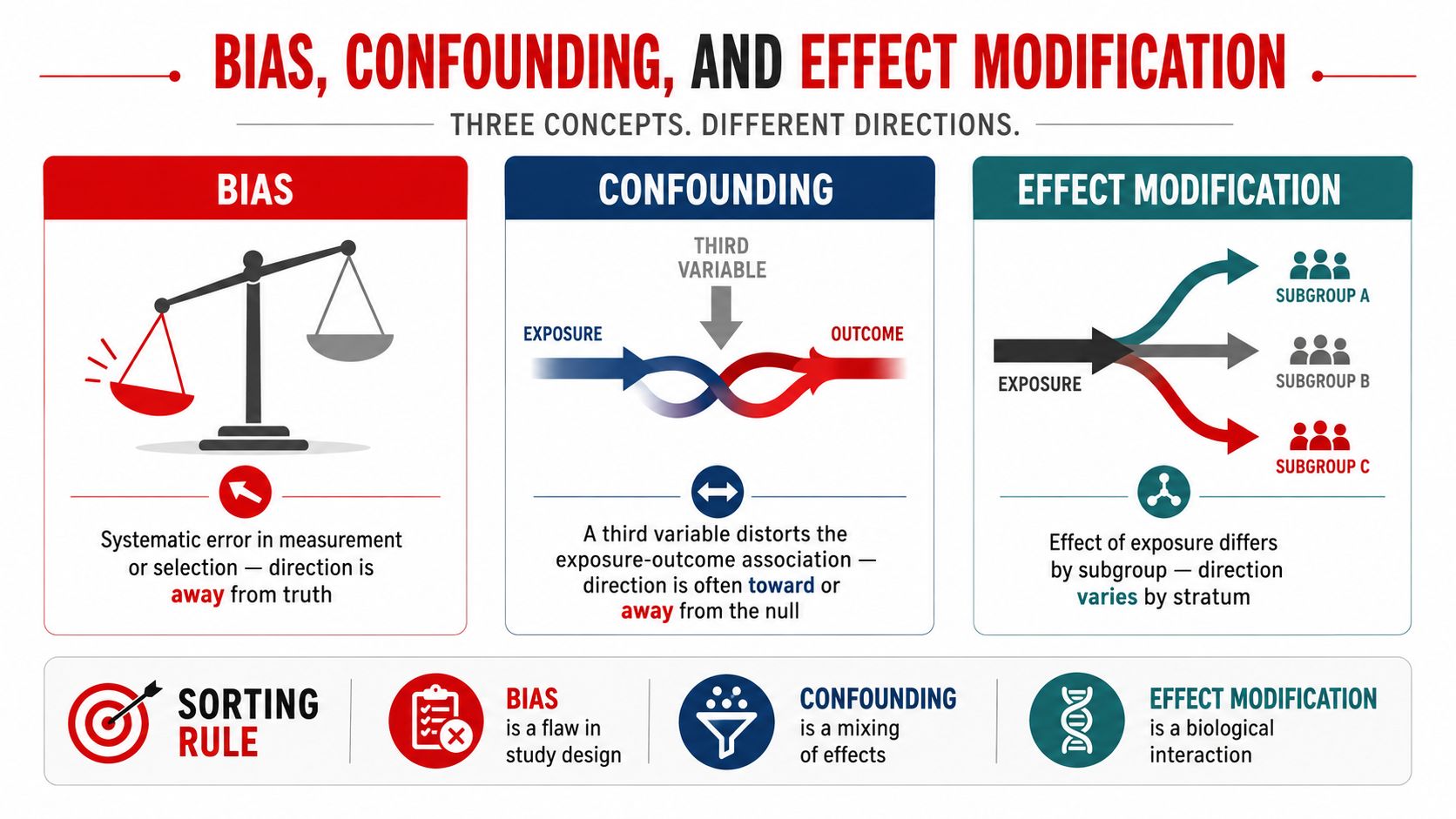
These terms describe different problems. Bias is systematic error introduced by how a study selects participants or measures information. Confounding is distortion caused by a third variable. Effect modification means the exposure effect differs across subgroups.
Sort the direction of the problem
Selection bias occurs when inclusion, exclusion, participation, or loss to follow-up changes the relationship between exposure and outcome. The healthy worker effect is a classic example: employed people may differ systematically from the general population, making an occupational exposure appear less harmful than it is.
Information bias occurs when investigators measure exposure or outcome inaccurately. Recall bias can arise when people with disease remember past exposures differently from controls. Interviewer bias can occur when an investigator's expectations influence how information is collected. Differential misclassification means the measurement error differs between groups.
Confounding requires three features:
- The third variable is associated with the exposure.
- It is independently associated with the outcome.
- It isn't on the causal pathway between exposure and outcome.
Researchers can address confounding through restriction, matching, stratification, and multivariable regression. Randomization can also reduce confounding in an appropriately conducted trial because treatment assignment is determined by chance rather than participant characteristics.
Confounding is not effect modification
Effect modification isn't a flaw to eliminate. It means the exposure has different effects in different strata, so the investigator should report stratum-specific results rather than combine them into one adjusted estimate.
Consider a composite teaching case in which hormone replacement therapy appears protective against coronary heart disease in a crude analysis. After stratification by socioeconomic status, the association changes substantially because socioeconomic status is related to both treatment use and coronary risk. That pattern suggests confounding if socioeconomic status is not on the causal pathway.
If the therapy's effect differs across socioeconomic strata, however, socioeconomic status may be an effect modifier. The deciding question is whether stratification reveals distortion of one underlying effect or different effects across groups.
The selection bias explanation can reinforce the distinction between a flawed sampling process and a real subgroup difference. On an exam, ask whether the third variable should be controlled away or described as part of the result.
Screening, Surveillance, and Outbreak Investigation
Applied epidemiology turns measurement into action. Primary prevention prevents disease before it begins, such as immunization. Secondary prevention detects disease early through screening. Tertiary prevention limits complications after disease has developed.
Screening questions often test both test characteristics and program design. The classic Wilson-Jungner framework asks whether the condition matters, has an accepted treatment, has an available facility, includes a recognizable latent stage, and has a suitable and acceptable test. It also considers whether the natural history is understood, a policy exists for whom to treat, the cost is reasonable, and follow-up can continue.
Screening logic
Sensitivity and specificity are properties of the test in relation to disease status. Predictive values answer a different question, namely what a positive or negative result means in the tested population. Because predictive value depends on the underlying prevalence, a strong test can produce many false-positive results when used where disease is uncommon.
The CDC defines surveillance as the ongoing, systematic collection, analysis, interpretation, and dissemination of health data to guide public-health decisions and action. Its phrase “information for action” captures the point: surveillance isn't passive record-keeping. The CDC surveillance framework connects collected information to investigation, control, prevention, and communication.
Passive surveillance relies on routine reports submitted through existing systems. Active surveillance involves actively searching for cases, contacting reporting sites, or reviewing records to identify additional cases.
Outbreak investigation
The CDC describes a structured sequence of 13 outbreak-investigation steps. The opening steps include preparing for fieldwork, establishing whether an outbreak exists, and verifying the diagnosis. Depending on the situation, those first steps may occur in reverse order or simultaneously.
A practical condensed version is:
- Prepare for fieldwork.
- Establish that an outbreak exists.
- Verify the diagnosis.
- Create a workable case definition.
- Find additional cases.
- Build a line list or database.
- Describe cases by person, place, and time.
- Develop hypotheses.
- Evaluate hypotheses analytically.
- Refine hypotheses when needed.
- Implement control measures.
- Maintain surveillance.
- Communicate findings.
The CDC outbreak investigation summary emphasizes case definitions, systematic case finding, line lists, duplicate checking, and cohort or case-control studies. For broader infection-prevention context, review infection control protocols.
Practice prompt: If several people develop cholera after a community event, what information would you collect first? Name the population, suspected exposure, outcome definition, comparison group, and time window before choosing a study design.
Study Plan, Self-Audit, and Key Takeaways
Use a four-week sequence:
- Week 1: Disease frequency, incidence, prevalence, attack rate, and case fatality rate.
- Week 2: Study designs, 2×2 tables, relative risk, odds ratio, ARR, NNT, and NNH.
- Week 3: Bias, confounding, effect modification, and causal inference.
- Week 4: Screening, surveillance, outbreak investigation, and mixed timed blocks.
Readiness checklist
You should be able to derive or explain:
- Incidence
- Prevalence
- Cumulative incidence
- Incidence rate
- Attack rate
- Case fatality rate
- Cohort design
- Case-control design
- Cross-sectional design
- Randomized controlled trial
- Relative risk
- Odds ratio
- Absolute risk reduction
- Number needed to treat
- Number needed to harm
- Sensitivity
- Specificity
- Positive predictive value
- Negative predictive value
- Selection bias, information bias, confounding, and effect modification
After each 20-question block, record accuracy by subtopic. Tag every missed item as a mechanism error, a recall error, or a transfer error, then record whether timing affected the result and whether you could apply the concept to an unseen question.
Identify the question first. Design determines the measure. Calculation comes before interpretation.
Keep five ideas immediately available: design dictates measure, odds ratio approximates relative risk only when disease is rare, confounding changes the apparent association, bias reflects systematic error, and screening value depends partly on prevalence. Official exam materials, including current USMLE content outlines and sample questions, should guide the final scope of your review; exam policies and formats can change, so verify them directly before planning.
If epidemiology questions remain inconsistent, Ace Med Boards offers individualized USMLE and COMLEX tutoring that can focus on study design recognition, 2×2 calculations, bias analysis, and timed question review. Visit Ace Med Boards to learn more or schedule a free consultation about your preparation needs.